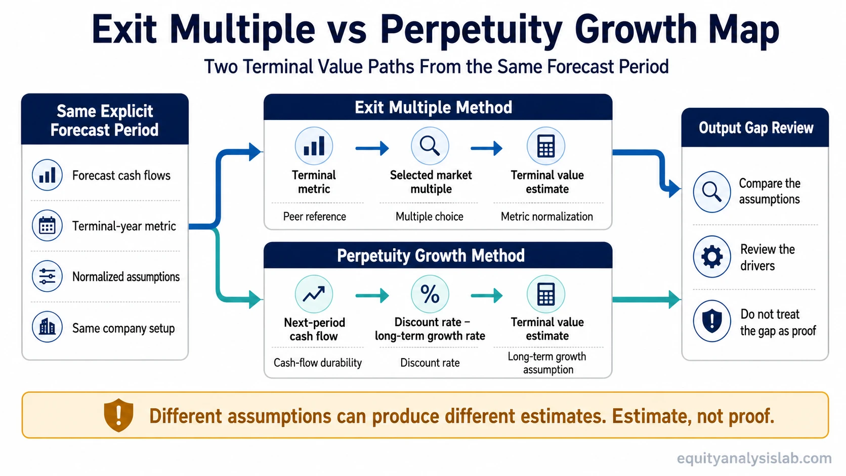
Exit multiple vs perpetuity growth compares two ways to estimate terminal value in a DCF valuation: exit multiple applies a market valuation multiple to a future financial metric, while perpetuity growth assumes cash flows continue growing at a sustainable long-term rate.
Both methods sit at the same point in the model, after the explicit forecast period. That shared location creates confusion. The difference is not only mathematical. Exit multiple asks what a business might be valued at using market-based multiples at the end of the forecast, while perpetuity growth asks what the continuing cash flows are worth under a long-run growth assumption.
Key points:
- Exit multiple uses a market multiple applied to a forecast metric such as EBITDA, EBIT, revenue, or another normalized measure.
- Perpetuity growth uses a continuing cash-flow assumption after the explicit forecast period.
- A gap between the two outputs is an assumption-review signal, not proof that either method is automatically correct.
What Exit Multiple vs Perpetuity Growth Means
The exit multiple method estimates terminal value by applying a valuation multiple to a financial metric expected near the end of the forecast period. The multiple is usually informed by peer valuations, transaction data, or market expectations for similar companies, though the final selection still requires judgment.
The perpetuity growth method estimates terminal value by assuming that cash flow continues beyond the explicit forecast period at a stable long-term growth rate. The long-term growth assumption is closely tied to the terminal growth rate, discount rate, reinvestment needs, and the company’s ability to sustain cash flows after the forecast period.
Core distinction: exit multiple is market-reference based; perpetuity growth is cash-flow-continuation based. Both can be used inside terminal value analysis, but they do not answer the same question.
Why the Two Methods Are Confused
Exit multiple and perpetuity growth are often confused because both appear after the final explicit forecast year. They can use the same revenue, margin, capital expenditure, working-capital, and cash-flow forecast before the terminal value step. A model can look identical until the final terminal value method changes.
The confusion becomes more important when the methods produce different values. A higher value from one method does not automatically make it more accurate. A lower value from the other method does not automatically make it more conservative. The difference usually shows that the terminal assumptions are telling different stories about the same company.
Confusion trap: same forecast inputs do not mean same valuation logic. The exit multiple method depends heavily on market multiple selection, while perpetuity growth depends heavily on the spread between the discount rate and the long-term growth assumption.
Key Differences Between Exit Multiple and Perpetuity Growth
| Comparison point | Exit multiple method | Perpetuity growth method |
|---|---|---|
| Question answered | What might the company be worth at the end of the forecast if valued using a market multiple? | What are the continuing cash flows worth if they grow at a sustainable long-term rate? |
| Primary input | A selected valuation multiple and a forecast metric, such as EBITDA, EBIT, revenue, or free cash flow. | A forecast cash flow, discount rate, and long-term growth assumption. |
| Data source | Market multiples, peer groups, precedent transactions, and comparable company valuation work. | Company cash-flow durability, reinvestment economics, long-run growth expectations, and discount-rate assumptions. |
| Best-fit context | Often more useful when relevant peer multiples exist and the terminal-year metric is normalized. | Often more useful when the central question is long-run cash-flow sustainability rather than market multiple comparison. |
| Main sensitivity | Highly sensitive to the selected multiple and the quality of the peer or transaction reference set. | Highly sensitive to small changes in long-term growth and discount rate assumptions. |
| Main weakness | Can import market optimism, pessimism, or peer-group mismatch into the valuation. | Can create large value changes from small assumption changes if growth and discount rate are close together. |
| Interpretation | Useful as a market-implied terminal value check, not a mechanical proof of value. | Useful as a cash-flow-continuity check, not a guarantee that the company can grow forever at the chosen rate. |
Same-Company Scenario: How the Outputs Can Diverge
Consider a generic company with a five-year forecast. The analyst projects revenue growth, margins, reinvestment needs, and free cash flow through the final forecast year. Up to that point, the model can be identical under both methods.
Illustrative setup: the company reaches a normalized terminal-year EBITDA level and produces positive free cash flow. Under the exit multiple method, the analyst applies a selected market multiple to the terminal-year EBITDA figure. Under the perpetuity growth method, the analyst takes the continuing cash flow and capitalizes it using the discount rate minus the long-term growth rate.
The exit multiple result may be higher if peer companies trade at elevated multiples or if the terminal metric looks especially strong. The perpetuity growth result may be lower if the long-term cash-flow growth assumption is modest or if the discount rate leaves a wide spread over growth.
The reverse can also happen. A conservative market multiple may produce a lower exit value, while a durable cash-flow profile with a defensible growth assumption may produce a higher perpetuity-growth value.
The useful conclusion is not that one method wins. The useful conclusion is that the gap identifies where assumptions need review: peer selection, terminal-year normalization, cash-flow durability, reinvestment burden, discount rate, and long-term growth.
When Exit Multiple Is More Defensible
Exit multiple is more market-reference dependent. It can be more defensible when the company has a clear peer set, the terminal-year metric is normalized, and the selected multiple is tied to companies with similar growth, margin, risk, capital intensity, and business quality. It is especially useful when the valuation question is partly about what the market might pay for a mature version of the business.
The method becomes weaker when the peer group is loose, cyclical metrics are taken at a peak or trough, the multiple is selected to force a preferred outcome, or the comparison ignores capital structure, margins, growth, and reinvestment differences.
Exit multiple limitation: a market multiple can reflect market mood as much as business economics. A clean peer group can support the assumption, but it cannot remove the need to test whether the terminal-year metric is representative.
When Perpetuity Growth Is More Defensible
Perpetuity growth is more explicit-assumption dependent. It can be more defensible when the company has relatively stable long-term cash-flow characteristics and the analyst wants to make the continuing-value assumption visible. The method forces attention onto sustainable growth, reinvestment needs, discount rate, and the economics required to support cash flow beyond the forecast period.
The method becomes weaker when the long-term growth rate is chosen casually, when cash flow is not normalized, or when the model assumes stable growth for a company whose economics are still highly cyclical, disrupted, or structurally uncertain.
Perpetuity growth limitation: small changes in the growth rate or discount rate can create large changes in terminal value. That sensitivity makes the method useful for assumption testing, but risky if the output is treated as precise.
Formula Note: Keep the Math as a Comparison Tool
The formulas are useful because they show why the methods behave differently, but the comparison should not become a formula walkthrough.
| Method | Simple expression | What drives the output |
|---|---|---|
| Exit multiple | Terminal metric × selected multiple | Metric quality, normalization, peer selection, and multiple choice. |
| Perpetuity growth | Next-period cash flow ÷ (discount rate − long-term growth rate) | Cash-flow durability, discount rate, growth assumption, and reinvestment economics. |
The formulas explain the sensitivity. They do not decide which estimate is right. For the perpetuity growth expression to be usable, the discount rate must be greater than the long-term growth rate; otherwise, the denominator does not support a defensible continuing-value estimate.
Common Mistakes When Comparing the Methods
Mistake 1: Averaging both values automatically. Averaging can hide the real disagreement between assumptions. If one method produces a much higher estimate, the reason for the gap should be reviewed before combining outputs.
Mistake 2: Treating the exit multiple as more practical by default. Market multiples can be useful, but they can also reflect a temporary valuation environment or a poor peer match.
Mistake 3: Treating perpetuity growth as more theoretical by default. The method is assumption-heavy, but it can be valuable when cash-flow durability is the main question and the assumptions are explicit.
Mistake 4: Letting terminal value dominate the model without review. If most of the valuation comes from terminal value, the terminal assumptions deserve more scrutiny than the headline output.
How to Read a Gap Between the Two Outputs
A large gap between exit multiple and perpetuity growth is not a clean answer. It is a diagnostic prompt. The analyst should ask which assumption is creating the difference and whether that assumption fits the company’s economics.
Output-gap diagnostic:
- If exit multiple is much higher, check whether peer multiples are elevated, the selected multiple is too generous, or the terminal metric is above normalized levels.
- If perpetuity growth is much higher, check whether the growth rate is too close to the discount rate or whether cash-flow durability is being overstated.
- If both methods produce similar values, do not assume the estimate is correct. Similar outputs can still come from weak assumptions.
- If both methods are highly sensitive, focus on assumption ranges instead of a single point estimate.
Related Valuation Concepts
Exit multiple and perpetuity growth are easiest to compare when the surrounding valuation concepts stay separate. Exit multiple belongs to market-multiple terminal value logic. Terminal growth rate belongs to long-run cash-flow continuation. Comparable company analysis helps explain where market multiples may come from. DCF valuation provides the broader framework where terminal value is estimated and discounted back to the present.
Keeping those concepts separate helps prevent a common modeling problem: using one terminal value number as if it were independent from the assumptions that created it.
FAQ
Is exit multiple better than perpetuity growth?
No. Exit multiple is not automatically better than perpetuity growth. It can be more defensible when relevant market multiples and normalized terminal metrics are available. Perpetuity growth can be more defensible when the central question is long-term cash-flow durability. The better method depends on the company, the available evidence, and the assumptions being tested.
Why do exit multiple and perpetuity growth produce different values?
They produce different values because they rely on different assumption sets. Exit multiple depends on a selected market multiple and terminal-year metric. Perpetuity growth depends on cash flow, discount rate, and long-term growth. A gap between the two estimates should be reviewed as an assumption difference, not treated as proof that one value is correct.
Should both terminal value methods be used together?
Both methods can be compared as a sensitivity check, but using both does not guarantee accuracy. The important step is understanding why the estimates agree or disagree. Averaging the outputs without reviewing the assumptions can hide the real valuation issue.